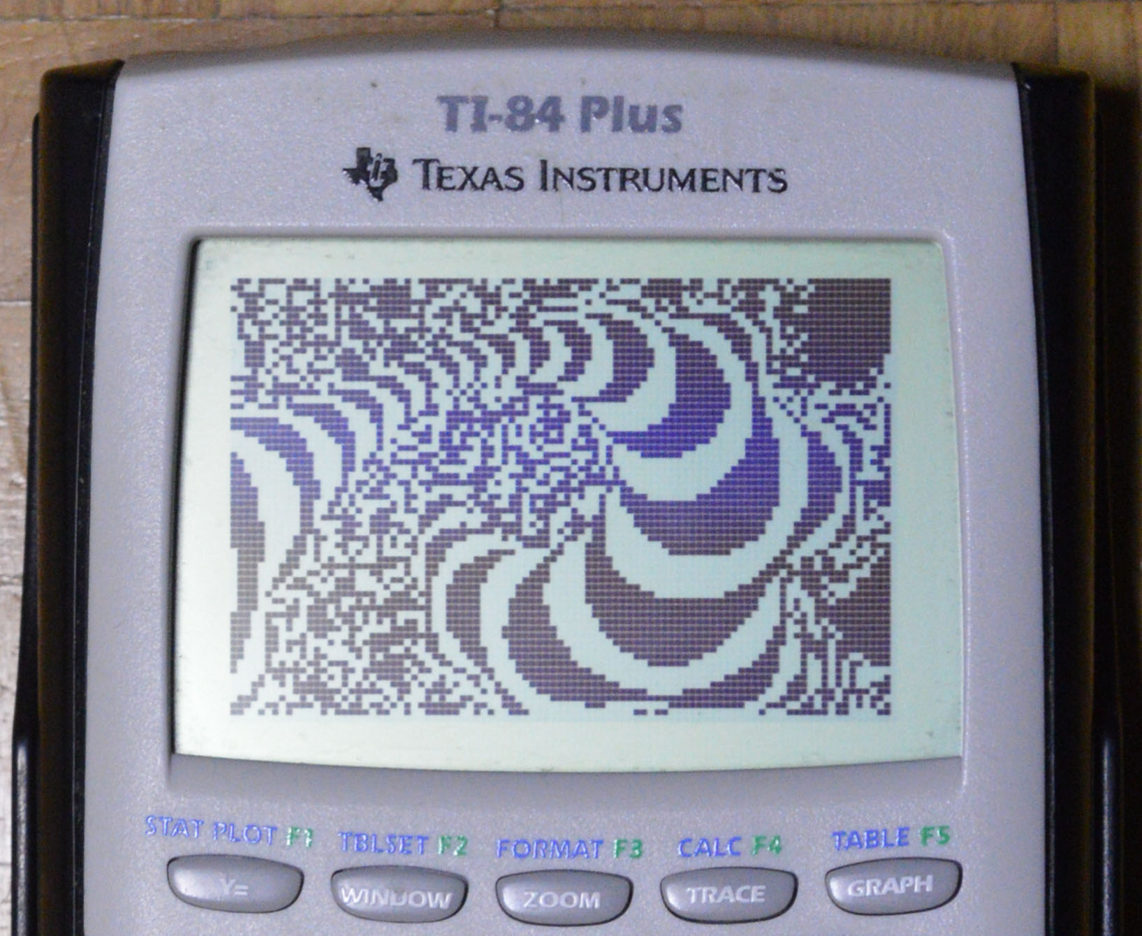
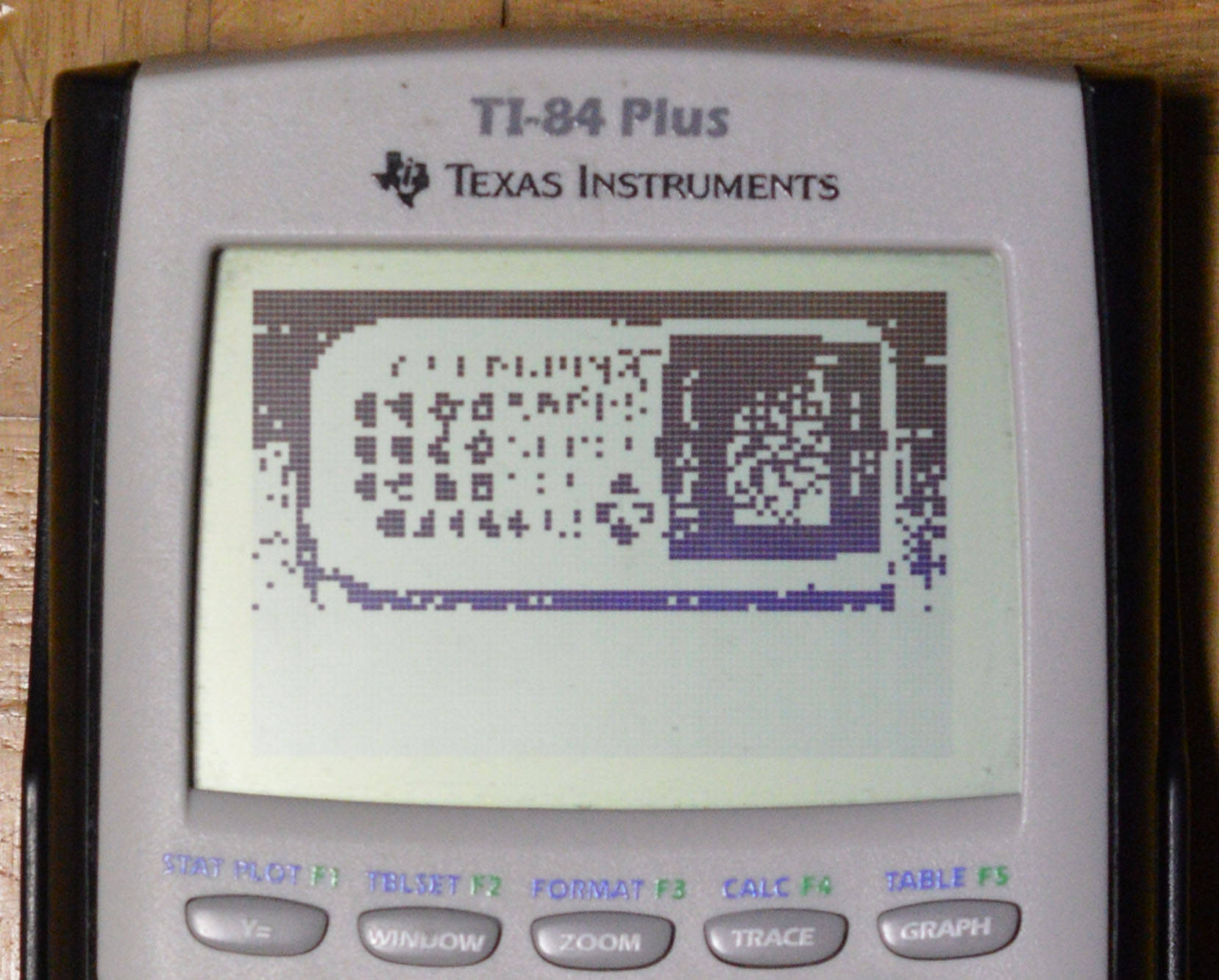
Christmas MMXVII
2017-12-25, post № 188
art, haiku, poetry, #fractal, #Mandelbrot set
Barren trees, white snow.
Cold and lasting winter nights.
Quiet fire crackling.
2017-12-25, post № 188
art, haiku, poetry, #fractal, #Mandelbrot set
Barren trees, white snow.
Cold and lasting winter nights.
Quiet fire crackling.
2017-12-16, post № 187
mathematics, programming, Python, #linear algebra, #matrices
Matrices are an important part of linear algebra. By arranging scalars in a rectangular manner, one can elegantly encode vector transformations like scaling, rotating, shearing and squashing, solve systems of linear equations and represent general vector space homomorphisms.
However, as powerful as matrices are, when actually applying the theoretical tools one has to calculate specific values. Doing so by hand can be done, yet gets cumbersome quite quickly when dealing with any matrices which contain more than a few rows and columns.
So, even though there are a lot of other implementations already present, I set out to write a Python matrix module containing a matrix class capable of basic matrix arithmetic (matrix multiplication, transposition, …) together with a set of functions which perform some higher-level matrix manipulation like applying Gaussian elimination, calculating the reduced row echelon form, determinant, inversion and rank of a given matrix.
Module source code can be seen below and downloaded. When saved as matrix.py in the current working directory, one can import the module as follows.
>>> import matrix
>>> A = matrix.Matrix([[13,  1, 20, 18],
...                    [ 9, 24,  0,  9],
...                    [14, 22,  5, 18],
...                    [19,  9, 15, 14]])
>>> print A**-1
        -149/1268  -67/634   83/1268 171/1268
          51/1268 239/1902 -105/1268 -33/1268
Matrix(    73/634 803/4755  -113/634 -87/3170 )
          13/1268  -75/634  197/1268 -83/1268
Matrices are defined over a field, typically [1] in theoretical use, though for my implementation I chose not to use a
double data structure [2], as it lacked the conceptual precision in numbers like a third [3]. As one cannot truly represent a large portion of the reals anyways, I chose to use , which also is a field though can be — to a certain scalar size and precision — accurately represented using fractional data types (Python’s built-in
Fraction is used here).
To simplify working with matrices, the implemented matrix class supports operator overloading such that the following expressions — A[i,j], A[i,j]=l, A*B, A*l, A+B, -A, A/l, A+B, A-B, A**-1, A**"t", ~A, A==B, A!=B — all behave in a coherent and intuitive way for matrices A, B, scalars l and indices i, j.
When working with matrices, there are certain rules that must be obeyed, like proper size when adding or multiplying, invertibility when inverting and others. To minimize potential bug track down problems, I tried to include a variety of detailed exceptions (ValueErrors) explaining the program’s failure at that point.
Apart from basic matrix arithmetic, a large part of my module centers around Gaussian elimination and the functions that follow from it. At their heart lies the implementation of GaussianElimination, a function which calculates the reduced row echelon form rref(A) of a matrix together with the transformation matrix T such that T*A = rref(A), a list of all matrix pivot coordinates, the number of row transpositions used to achieve row echelon form and a product of all scalars used to achieve reduced row echelon form.
From this function, rref(A) simply returns the first, rrefT(A) the second parameter. Functions rcef(A) (reduced column echelon form) and rcefS(A) (A*S = rcef(A)) follow from repeated transposition.
Determinant calculation uses characteristic determinant properties (multilinear, alternating and the unit hypercube has hypervolume one).
Using these properties, the determinant is equal to the product of the total product of all factors used in transforming the matrix into reduced row echelon form and the permutation parity (minus one to the power of the number of transpositions used).
Questions regarding invertibility and rank can also conveniently be implemented using the above described information.
All in all, this Python module implements basic matrix functionality paired with a bit more involved matrix transformations to build a usable environment for manipulating matrices in Python.
2017-12-02, post № 186
ImageMagick, PIL, programming, Python, #animation, #automation, #cellular, #PPCG, #quantum mechanics
A recent PPCG challenge titled The Quantum Drunkard’s Walk was about a tiny drunken person for which quantum mechanics apply and who — being drunk — will randomly walk in one of the four cardinal directions each step they take.
As they experience the strange world of quanta, they can simultaneously take every path at once and their paths influence each other. The challenge then asked to output all possible positions the quantum drunkard could occupy, all paths they could take in ASCII representation.
The question also states this problem’s equivalence to a cellular automaton, when one removes the story boilerplate.
Cells in this cellular automaton are square and can occupy one of three states: empty, awake or sleeping. Each iteration, all cells change according to three rules.
Being code golf, the aim was to come up with a minimally sized source code; my attempt required 𝟤𝟣𝟦 bytes and prints a nested array containing one-length strings (characters), as this output method is cheaper than concatenating all characters to one string.
However, one user took the challenge idea a bit further and created an animated gif showing the walk’s, or cellular automaton’s, progression over time with an increasing number of iterations. My Python program shown in this post does exactly that, generating an animated gif showing the automaton’s progression. I even implemented rainbow support, possibly improving the automaton’s visual appearance.
Python source code can be downloaded and seen below.
I use the Python Imaging Library to produce all frames and use a shell call to let ImageMagick convert all frames to an animated gif. Animation parameters are taken via shell arguments, a full list of features follows (also available via the -h flag).
--iterations N: Number of iterations (initial frame not counted)--colorempty C: Empty cell color (#rrggbb)--colorawake C: Awake cell color (#rrggbb)--colorsleeping C: Sleeping cell color (#rrggbb)--rainbow: Use rainbow colors (overrides color settings)--scale N: Cell square pixel size--convert: Execute ImageMagick’s convert command--delay N: Delay between frames in output image.--loop N: Gif loops (0 means for indefinite looping)--keepfiles: Do not delete files when converting2017-11-18, post № 185
art, haiku, poetry,
A tiny spark flies;
Ignites a crumbled paper.
Thus fire is born.
2017-11-04, post № 184
C, programming, Python, #recreational
A polyglot — coming from the Greek words πολύς (many) and γλώττα (tongue) — is a piece of source code which can run in multiple languages, often performing language-dependent tasks.
Even though such a source code’s feature may not seem particularily useful or possible with certain language combinations, trying to bend not one but multiple language’s syntactic rules and overall behavior is still interesting.
An example of a rather simple polyglot would be a Python 2 / Python 3 polyglot — if one counts those as two separate languages. Because of their enormous similarities, one can pick out differences and use those to determine which language runs the source code.
if 1/2>0:print("Python 3")
else:print("Python 2")
Utilizing Python’s version difference regarding integer division and real division is one of the most common ways to tell them apart, as it can also be used to only control a specific part of a program instead of having to write two nearly identical programs (increases the program’s style and cuts on bytes — an important consideration if one golfs a polyglot).
However, polyglots combining languages that are not as similar as Python 2 and Python 3 require more effort. The following is a general Python 2 / C polyglot, meaning that nearly all C and Python 2 programs can be mixed using this template (there are a few rules both languages need to abide which will come apparent later).
#define _\
"""
main(){printf("C");}
#define _"""
#define/*
print"Python 2"
#*/_f
In the above code, main(){printf("C");} can be nearly any C code and print"Python 2" can be nearly any Python 2 code.
Language determination is exclusively done via syntax. A C compiler [1] sees a #define statement and a line continuation \, another two #define statements with a block comment in between and actual compilable C source code (view first emphasis).Python, on the other hand, treats all octothorps, #, as comments, ignoring the line continuation, and triple-quoted strings, """...""", as strings rather than statements and thus only sees the Python code (view second emphasis).
My first ever polyglot used this exact syntactical language differentiation and solved a task titled Life and Death of Trees (link to my answer).
2017-10-31, post № 183
art, poetry, #dark, #iambic pentameter, #poem, #Shakespearean sonnet, #sonnet
— Jonathan Frech, 30th of October 2017
Manuscript.
2017-10-21, post № 182
C, programming, #bitmap, #file, #file format
C is one cool and important language. CPython and Unix are based on it, the Mars Curiosity rover is run by it and even the GCC C compiler itself is written in C. However, as C is some years old by now, it lacks a lot of higher-level features most modern languages possess, being more down to the silicon, as the cool kids say. Concepts like pointer manipulation, bit fiddling and its string implementation — just to name a few — are at times cumbersome, insecure and error-prone; nevertheless is there a certain appeal to writing in C.
Being only one abstraction level away from Assembly — which itself is only one abstraction level above raw byte code — and having access to file manipulation down to the individual bit, I set out to write a Microsoft Bitmap (.bmp) implementation in pure C. As Microsoft’s standard for this image file format is quite feature-rich, I decided to focus on the bare minimum — a bitmap with 𝟤𝟦-bit color depth (three colors, one byte per), one color plane, no compression, no palette and 𝟥𝟢𝟢 DPI.
My Bitmap implementation supports both reading and writing .bmp files, as well as generating some test images — including a Mandelbrot set fractal renderer, of course. Implementation source code can be downloaded (bmp.c) or seen below.
Implementing a file format requires knowing its specification. Although it is not the best article I have ever seen, this Wikipedia article gave me some insights. The missing pieces were reverse engineered using Adobe Photoshop CC and the HxD hex editor.
The following is a snippet of the implementation’s savebmp function (full source code listed below). It illustrates the Bitmap file’s byte layout only showing the file header, omitting a lengthy data part concatenated to the header. S, K, W, H and B are all byte arrays of length four (little-endian format) which contain the file’s total size, the bitmap data offset (which is constant, since the header is always exactly 𝟧𝟦 bytes large), the image’s dimensions (horizontal and vertical) and the bitmap data’s section’s size, respectively.
/*  bitmap file header  */
0x42, 0x4D,             // BM
S[0], S[1], S[2], S[3], // file size
0x00, 0x00, 0x00, 0x00, // unused
K[0], K[1], K[2], K[3], // bitmap data offset
/*      DIB header      */
0x28, 0x00, 0x00, 0x00, // DIB size
W[0], W[1], W[2], W[3], // pixel width
H[0], H[1], H[2], H[3], // pixel height
0x01, 0x00,             // one color plane
0x18, 0x00,             // 24 bit color depth
0x00, 0x00, 0x00, 0x00, // no compression
B[0], B[1], B[2], B[3], // bitmap data size
0x23, 0x2E, 0x00, 0x00, // 300 DPI (horizontal)
0x23, 0x2E, 0x00, 0x00, // 300 DPI (vertical)
0x00, 0x00, 0x00, 0x00, // no palette
0x00, 0x00, 0x00, 0x00  // color importance
/*  data bytes follow   */
Key bytes to note are the first two identifying the file type (the ASCII-encoded letters BM) and the DPI bytes, 0x23, 0x2E, which indicate 0x00002E23 = 11811 pixels per meter in both the horizontal and vertical direction. Converting from pixels per meter to dots per inch results in 11811 / (1 meter / 1 inch) = 11811 * 127 / 5000 = 300 DPI (roughly).
Most values are represented using four bytes in little-endian format. Translating an 𝟥𝟤-bit integer into four little-endian formatted bytes can be achieved as follows.
/* unsigned 32-bit integer */
unsigned int n = 0b10100100010000100000100000010000;
/*                 < m sig><sm sig><sl sig>< l sig> */

/* byte (unsigned char) array of size four */
unsigned char N[4] = {
    (n & 0xff000000) >>  0, // most significant byte
    (n & 0x00ff0000) >>  8, // second most significant byte
    (n & 0x0000ff00) >> 16, // second least significant byte
    (n & 0x000000ff) >> 24  // least significant byte
};
Other than rendering a fractal, I also implemented three nested loops which output an image containing every possible color exactly once ((2**8)**3 = 16777216 pixels in total).
An image’s data type is implemented as a struct image which contains three variables — width and height, two integers specifying the image’s dimensions, and *px, a pointer to an one-dimensional integer array of size width*height which holds the entire image data.
Defined functions are listed ahead.
image * readbmp(char []); Reads an image specified by a file name. If reading fails, a NULL pointer is returned.void savebmp(image *, char []); Saves given image to a file with specified name.image * newimage(int, int); Returns a pointer to an image struct with specified dimensions (image will be filled with nothing but black pixels).void freeimage(image *); Frees an image struct’s memory.int getpx(image *, int, int); Returns the pixel color at specified coordinates.void setpx(image *, int, int, int); Sets the pixel color at specified coordinates.void fill(image *, int); Fills a given image with a given color (all pixels are set to specified color).int color(byte, byte, byte); Returns a 𝟥𝟤-bit integer representing a color specified by three bytes (byte is defined through typedef unsigned char byte;(.int hsl(double, double, double); Returns a 𝟥𝟤-bit integer representing a color specified by three doubles in the HSL color format.Images shown in this post were converted to .png files as WordPress does not allow .bmp file uploads; the raw pixel data should, however, be identical. [1]
2017-10-07, post № 181
BASIC, PIL, programming, Python, TI-84 Plus, #bitmap, #image, #TI, #TI-BASIC
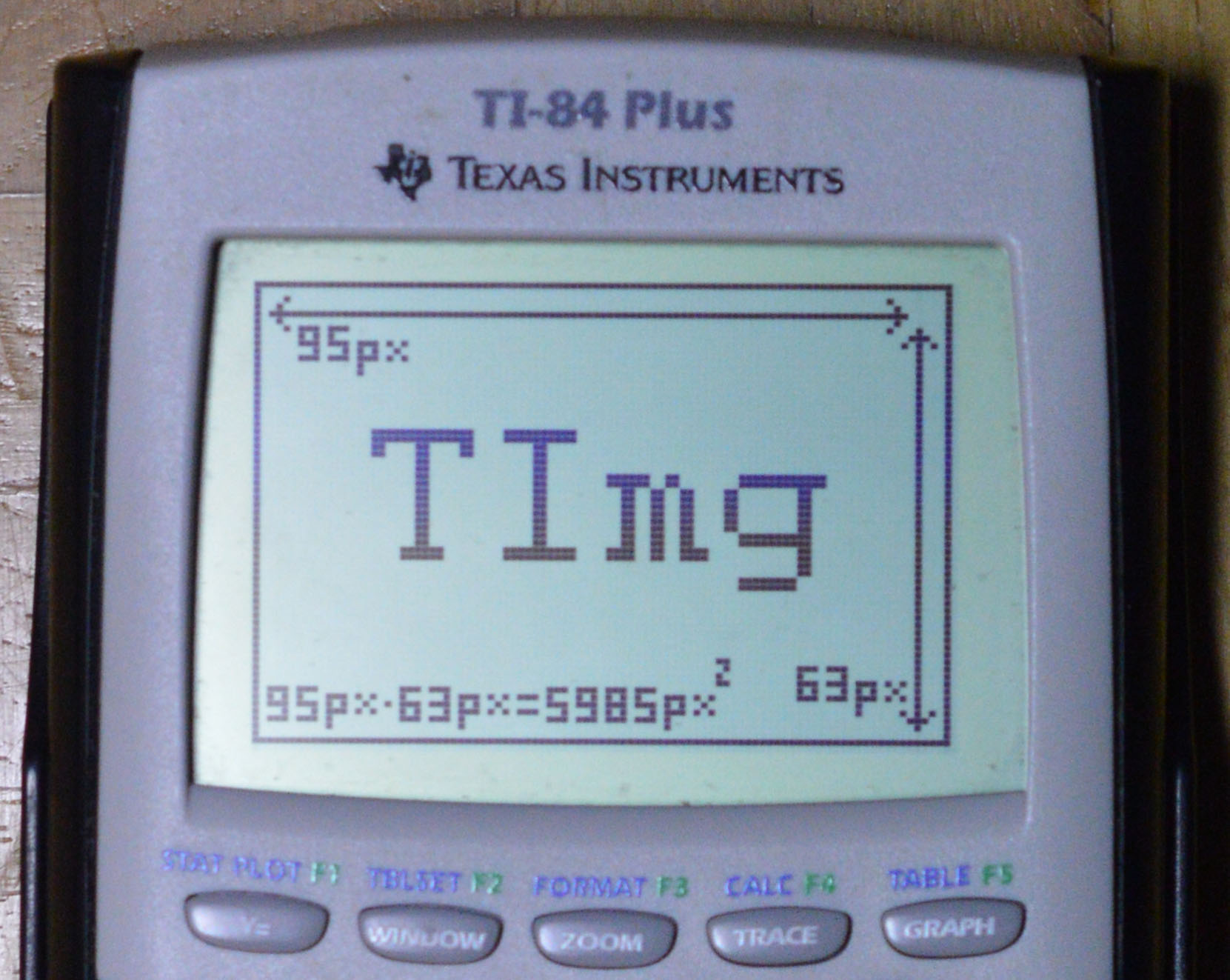
Texas Instrument’s TI-84 Plus is a graphing calculator with a variety of features. It has built-in support for both fractions and complex numbers, can differentiate and integrate given functions and supports programming capabilities. The latter allows to directly manipulate the calculator’s monochrome display’s 𝟧𝟫𝟪𝟧 pixels (the screen has dimensions 𝟫𝟧 ⨉ 𝟨𝟥). TImg is a Python program (source code is listed below and can also be downloaded) which takes in an image and outputs TI-BASIC source code which, when run on the graphing calculator, will produce the given image — in potentially lower quality.

PIL — the Python Imaging Library — is used to read in the image and further for processing. The supplied image may be rotated and resized to better fit the TI-84’s screen and any color or even grayscale information is reduced to an actual bitmap — every pixel only has two distinct values.
Direct pixel manipulation on the TI-84 is done via the Graph screen. To get remove any pixels the system draws on its own, the first three commands are ClrDraw, GridOff and AxesOff which should result in a completely blank screen — assuming that no functions are currently being drawn. All subsequent commands are in charge of drawing the previously computed bitmap. To turn certain pixels on, Pxl-On(Y,X is used where 𝑌 and 𝑋 are the pixel’s coordinates.

Since the TI-84 Plus only has 𝟤𝟦 kilobytes of available RAM, the source code for a program which would turn on every single pixel individually does not fit. Luckily, though, a program which only individually turns on half of the screen’s pixels fits. To ensure that TImg’s output fits on the hardware it is designed to be used with, an image’s bitmap is inverted when the required code would otherwise exceed 𝟥𝟧𝟢𝟢 lines — a value slightly above the required code to draw half of the pixels.
